Setting & model

Online Bipartite Matching

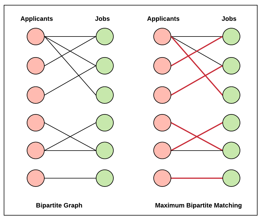
The author Karp, Vazirani, and Vazirani introduce a bipartite graph model $G =(U \cup V, E)$, where $U$ is given offline and $V$ arrives online [KVV90]. The online algorithm must irrevocably match each arriving vertex $v \in V$ to an unmatched neighbor in $U$ or leave it unmatched.

The offline optimal is defined as the maximum matching in $G$. The competitive ratio is defined as the expected size of the matching produced by the online algorithm divided by the size of the offline optimal matching.

$$Ratio = ALG / OPT$$

Online Stochastic Matching Problem

In the online matching problem with stochastic rewards, every edge $(u, v)$ also has an associated probability of success $p_{uv}$.

When a new vertex $v \in V$ arrives online, the algorithm either chooses not to assign it at all, or assigns it to one of its neighbors (these are the available options).

If $v$ is assigned to $u \in U$ using the edge $(u, v)$, a Bernoulli experiment is performed and the edge $(u, v)$ becomes a successful assignment with probability $p_{uv}$.

In successful assignment case, we say that $u$ was successful and remove it from the set of available vertices. On the other hand, if the assignment $(u, v)$ is not successful, $u$ remains available and a neighbor of $u$ that arrives later in the online order can be assigned to $u$ (but $v$ cannot be assigned in the future).

The overall objective is to maximize the expected number of successful vertices $u \in U$, or equivalently, the expected number of successful assignments.

Vertex-Weighted Stochastic Matching

In the vertex-weighted variant, each offline vertex $u \in U$ has a nonnegative weight $w_u$. A successful assignment on $u$ yields reward $w_u$ and removes $u$ from availability (as before). The objective becomes maximizing the expected total weight of successful offline vertices:

$$\max \mathbb{E} \left[\sum_{u \in U} w_u \cdot \mathbf{1}\{u\ \text{is matched successfully}\}\right].$$

The unweighted model is the special case $w_u \equiv 1$.

The four probability regimes below (Vanishing/Arbitrary × Equal/Unequal) remain the same; results in recent work typically extend to the vertex-weighted case with essentially the same analyses.

Probability Settings

1. Vanishing & Equal Probabilities
2. Vanishing & Unequal Probabilities
3. Arbitrary/Non-Vanishing & Equal Probabilities
4. Arbitrary/Non-Vanishing & Unequal

Offline Optimal Benchmark

The Budgeted Allocation Problem

Let $G = (U \cup V, E)$ be a bipartite graph where edge $(u, v)$ has weight $p_{uv}$. For every vertex $v \in V$, we assign it to one its neighbors $u \in U$ using edge $(u, v)$. The load $L_u$ on a vertex $u \in U$ is defined as the sum of weights of assigned edges incident on $u$. The objective is to maximize $\sum_{u \in U} \min(L_u, 1)$.

For technical reasons, we allow fractional solutions, i.e. vertex $v \in V$ can be assigned to its neighbors $u \in U$ with fractions $x_{uv}$ subject to $\sum_{u \in U} x_{uv} \le 1$; then $L_u = \sum_{u \in U} x_{uv} p_{uv}$.

For any instance of the Online Stochastic Matching problem, we define $OPT$ to be the optimum fractional solution for the corresponding Budgeted Allocation problem. The next lemma claims that the value of $OPT$ is at least the expected number of successes obtained by any Online Stochastic Matching algorithm.

Distribution of the Success Threshold (Ө)

Let $\tau$ be the round of the first success when repeatedly attempting the same offline vertex $u$. Then

$$\tau \sim \operatorname{Geom}(p) \quad(\tau=1,2,3, \ldots) .$$

Measure “load” as the cumulative success probability: each attempt adds $p$. Define

$$\Theta:=p \cdot \tau .$$

Hence,

$$\operatorname{Pr}[\Theta=t p]=p(1-p)^{t-1} \quad(t=1,2, \ldots)$$

so $\Theta$ only takes values in $\{p, 2 p, 3 p, \ldots\}$. A vertex $u$ becomes successful the first time its accumulated load $\ell_u$ reaches or exceeds $\Theta$. This is exactly the “equivalent threshold view” used by Mehta-Panigrahi.

Basic moments. $\mathbb{E}[\Theta]=1$ and $\operatorname{Var}(\Theta)=1-p$. Thus, as $p \rightarrow 0$, both the mean and the variance tend to 1.

Vanishing limit $(p \rightarrow 0)$. Viewing the discrete distribution as a continuous-load approximation,

$$\operatorname{Pr}[\Theta>x]=(1-p)^{\lfloor x / p\rfloor} \underset{p \rightarrow 0}{\longrightarrow} e^{-x}$$

i.e., $\Theta \Rightarrow \operatorname{Exp}(1)$. Consequently, in small-$p$ analyses it is standard to model each offline vertex’s threshold as an independent $\operatorname{Exp}(1)$ random variable.

Unequal but small probabilities. If the edge success probabilities $p_{u v}$ differ but are all small, we still measure load as the sum of allocated success probabilities. In this continuous-load coordinate, the threshold is well-approximated by $\operatorname{Exp}(1)$; each attempt just increments the load by the corresponding $p_{u v}$ instead of a fixed $p$.

Definition of Competitive Ratio

Let $N_u$ denote the set of neighbors of an offline vertex $u$.

For the unweighted case, the competitive ratio is $\mathbb{E}[ALG]/OPT$.

For the vertex-weighted case, the competitive ratio is $\mathbb{E}[ALG_w]/OPT_w$.

A convenient upper bound/benchmark is the (configuration) LP relaxation; a simple edge-based LP that suffices for exposition is:

$$\begin{aligned} \max \quad & \sum_{u \in U} w_u\cdot p_{uv} \cdot x_{uv} \\ \text{s.t.}\quad & \sum_{v \in N(u)} p_{uv}\, x_{uv} \le 1 \qquad && \forall u \in U && (1) \\ & \sum_{u \in N(v)} x_{uv} \le 1 \qquad && \forall v \in V && (2) \\ & 0 \le x_{uv} \end{aligned}$$

Here $x_{uv}$ is the (fractional) probability of attempting $(u,v)$, all $w_u\equiv 1$ recovers the unweighted benchmark.

Eqn. (1) states that the expected load of each offline vertex $u$ is upper bounded by 1, because it is upper bounded by the expectation of the threshold $\theta_u$, which equals 1. (this uses the Law of Total Probability)

Eqn. (2) is a standard capacity constraint: each online vertex $v$ can be matched to at most one offline neighbor.

Following the vertex-weighted model of Mehta and Panigrahi [24], we will consider the optimal objective of the above LP relaxation as the benchmark.

Configuration LP

For any $S \subseteq N_u$, let $p_u(S)= \min \left\{\sum_{v \in S} p_{u v}, 1\right\}$. Consider the following offline-side configuration LP:

$$\begin{aligned} \text{ConfigLP:} \quad \max \quad & \sum_{u \in U} \sum_{S \subseteq N_u} w_u \cdot p_u(S) \cdot x_{u S} \\ \text{s.t.} \quad & \sum_{S \subseteq N_u} x_{u S} \leq 1 && \forall u \in U \\ & \sum_{u \in U} \sum_{S \subseteq N_u: v \in S} x_{u S} \leq 1 && \forall v \in V \\ & x_{u S} \geq 0 && \forall u \in U, \forall S \subseteq N_u \end{aligned}$$

From an offline optimization viewpoint, as $p$, the upper bound of success probabilities, tends to zero, the configuration LP is equivalent to the standard matching LP in the following sense. First, the matching LP can be reinterpreted as to maximize

$$\sum_{u \in U} w_u \cdot \min \left\{\sum_{v:(u, v) \in E} p_{u v} x_{u v}, 1\right\}$$

subject to only Eqn. (2) and (3).

On one hand, any feasible assignment of the configuration LP corresponds to a feasible assignment of the matching LP with

$$x_{u v}=\sum_{S \in N_u: v \in S} x_{u S}.$$

Comparing the objectives of the LPs, the matching LP objective is weakly larger because $\min \{z, 1\}$ is concave.

On the other hand, given any feasible assignment of the matching LP, we can sample an integral matching via independent rounding, i.e., match each online vertex $v$ to a neighbor that is independently sampled according to $x_{u v}$ ‘s.

Then, it gives an integral assignment of the configuration LP: $x_{u S}=1$ for the subset $S$ of neighbors matched to $u$ in the independent rounding, and 0 otherwise. Further, by standard concentration inequalities (and union bound), the load of each vertex $u$ is at most its expected load, which is at most 1 due to Eqn. (1), plus an additive error that diminishes as $p$ tends to zero. Hence, the optimal of the configuration LP is at least that of the matching LP less a term that diminishes as $p$ tends to zero.

The corresponding dual LP of the configuration LP is the following:

$$\begin{aligned} \text{Dual:} \quad \min \quad & \sum_{u \in U} \alpha_u+\sum_{v \in V} \beta_v \\ \text{s.t.} \quad & \alpha_u+\sum_{v \in S} \beta_v \geq w_u \cdot p_u(S) && \forall u \in U, \forall S \subseteq N_u \\ & \alpha_u, \beta_v \geq 0 && \forall u \in U, \forall v \in V \end{aligned}$$

An algorithm is $\Gamma$-competitive if:

1. Equal primal and dual objectives:

$$\sum_{u \in U} \sum_{S \subseteq N_u} p_u(S) \cdot w_u \cdot x_{u S}=\sum_{u \in U} \alpha_u+\sum_{v \in V} \beta_v ;$$

Approximate dual feasibility: For any $u \in U$ and any $S \subseteq N_u$,

$$\mathbf{E}\left[\alpha_u+\sum_{v \in S} \beta_v\right] \geq \Gamma \cdot w_u \cdot p_u(S)$$

Analyses

Let $\ell_u$ denote the load of an offline vertex $u \in U$, $\Theta$ be the vector of $\Theta_u$ for all $u \in U$, and let $\Theta_{-u}$ denote the entire vector $\Theta$ except $\Theta_u$.

For any fixed $(n-1)$-dimensional vector $\theta_{-u}$, let $\ell_u^{\infty}(\theta_{-u})$ be the load on vertex $u$ when $\Theta_{-u}=\theta_{-u}$ and $\Theta_u=\infty$ (i.e., in the “phantom world” where $u$ never succeeds).

Dual Assignment

Note that $u$‘s load increases over time; let $\ell_u$ denote the current load in the following discussion. For some non-decreasing function $f: \mathbf{R}^{+} \mapsto \mathbf{R}^{+}$ to be determined in the analysis, we maintain the dual assignment as follows:

1. Initially, let $\alpha_u=0$ for all $u \in U$.
2. On the arrival of an online vertex $v \in V$ and, thus, the corresponding dual variable $\beta_v$:
   • (a) If $v$ is matched to $u \in U$, increase $\alpha_u$ by $p \cdot f\left(\ell_u\right)$ and let $\beta_v=p\left(1-f\left(\ell_u\right)\right)$.
   • (b) If $v$ has no unsuccessful neighbor, let $\beta_v=0$.

Let $F(\ell)=\int_0^{\ell} f(z) \d z$ denote the integral of $f$. Note that we have $\alpha_u=F\left(\ell_u\right)$ in the limit as $p$ tends to zero.

Contribution from $\alpha_u$.
We now proceed to prove approximate dual feasibility using the above characterization. First, consider the contribution from the offline vertex $u$.

_For any thresholds $\theta_{-u}$ of offline vertices other than $u$ and the corresponding $\ell_u^{\infty}$:_

$$\mathbb{E}_{\theta_u}\!\left[\alpha_u \mid \theta_{-u}\right] \ge \int_{0}^{\ell_u^{\infty}} e^{-\theta_u}\, f(\theta_u)\, \d\theta_u \, .$$

By the above characterization, $u$‘s load equals $\ell_u^{\infty}$ when $\theta_u \ge \ell_u^{\infty}$, and equals $\theta_u$ when $0 \le \theta_u < \ell_u^{\infty}$. Further, recall that $\alpha_u = F(\ell_u)$ and that $\theta_u \sim \operatorname{Exp}(1)$. We get that:

$$\mathbb{E}_{\theta_u}\!\left[\alpha_u \mid \theta_{-u}\right] \ge \int_{0}^{\ell_u^{\infty}} e^{-\theta_u} F(\theta_u)\, \d\theta_u + e^{-\ell_u^{\infty}} F(\ell_u^{\infty}) = \int_{0}^{\ell_u^{\infty}} e^{-\theta_u} f(\theta_u)\, \d\theta_u \, .$$

Here, the equality follows by integration by parts. $\square$

---

Contribution from $\beta_v$’s.
Next, consider the contribution from the online vertices $v \in S$. For ease of notations, we let $z^{+}$ denote $\max\{z,0\}$.

For any thresholds $\theta_{-u}$ of offline vertices other than $u$ and the corresponding $\ell_u^{\infty}$:

$$\begin{aligned} \mathbb{E}_{\theta_u}\!\left[\sum_{v\in S} \beta_v \,\middle|\, \theta_{-u}\right] \ge &\left( e^{-\ell_u^{\infty}}\, p_u(S) + \int_{0}^{\ell_u^{\infty}} e^{-\theta_u}\, \big( p_u(S) - (\ell_u^{\infty}-\theta_u)^{+} \big)\, \d\theta_u \right) \\ &\times \big(1 - f(\ell_u^{\infty})\big)\, . \end{aligned}$$

Proof. By the above characterization, all vertices $v \in S$ are matched to neighbors with load at most $\ell_u^{\infty}$ at the time of the matches when $\theta_u \ge \ell_u^{\infty}$. This happens with probability $e^{-\ell_u^{\infty}}$ and contributes:

$$e^{-\ell_u^{\infty}}\, p_u(S)\cdot \big(1 - f(\ell_u^{\infty})\big),$$

to the expectation in the lemma.

Similarly, all vertices $v \in S$, except for $p^{-1}(\ell_u^{\infty}-\theta_u)$ of them, are still matched to neighbors with load at most $\ell_u^{\infty}$ at the time of the matches when $0 \le \theta_u < \ell_u^{\infty}$.

In the Stochastic Balance algorithm, each online vertex is matched to the unsuccessful neighbor with the least load, so only the overflow load $\ell_u^{\infty}-\theta_u$ exceeds $\theta_u$ and causes $u$ to become successful.

This contributes:

$$\int_{0}^{\ell_u^{\infty}} e^{-\theta_u}\, \big( p_u(S) - (\ell_u^{\infty}-\theta_u)^{+} \big)\, \d\theta_u \cdot \big(1 - f(\ell_u^{\infty})\big),$$

to the expectation. $\square$

So we have:

$$\mathbf{E}\left[\alpha_u+\sum_{v \in S} \beta_v\right] \geq \int_0^{\ell_u^{\infty}} e^{-\theta_u} f\left(\theta_u\right) \d \theta_u+\left(e^{-\ell_u^{\infty}} p_u(S)+\int_0^{\ell_u^{\infty}} e^{-\theta_u}\left(p_u(S)-\left(\ell_u^{\infty}-\theta_u\right)\right)^{+} \d \theta_u\right)\left(1-f\left(\ell_u^{\infty}\right)\right)$$

To show approximate dual feasibility, it suffices to find a non-decreasing function $f$ such that for any $\ell_u^{\infty} \geq 0$ and any $0 \leq p_u(S) \leq 1$ :

$$\int_0^{\ell_u^{\infty}} e^{-\theta_u} f\left(\theta_u\right) \d \theta_u+\left(e^{-\ell_u^{\infty}} p_u(S)+\int_0^{\ell_u^{\infty}} e^{-\theta_u}\left(p_u(S)-\left(\ell_u^{\infty}-\theta_u\right)\right)^{+} \d \theta_u\right)\left(1-f\left(\ell_u^{\infty}\right)\right) \geq \Gamma \cdot p_u(S)$$

Therefore, there is at most one index $j$ such that $\ell_j<\ell_u^{\infty}$ and $\ell_{j+1} \geq \ell_u^{\infty}$.

Solving the Differential Inequality

For ease of notations, we write $\ell_u^{\infty}$ as $\ell$, $p_u(S)$ as $p$, and $\theta_u$ as $\theta$. The dual feasibility inequality becomes:

$$\int_0^{\ell} e^{-\theta} f(\theta) \d \theta+\left(e^{-\ell} p+\int_0^{\ell} e^{-\theta}(p-(\ell-\theta))^{+} \d \theta\right)(1-f(\ell)) \geq \Gamma \cdot p .$$

First, note that the $z^{+}$ operation effectively restricts the second integration in the above equation to be from $\max \{0, \ell-p\}$ to $\ell$. This allows us to simplify by splitting into two cases.

Case 1: When $0 \leq p < \ell$, we need:

$$\int_0^{\ell} e^{-\theta} f(\theta) \d \theta+(1-f(\ell))\left(e^{-\ell+p}-e^{-\ell}\right) \geq \Gamma \cdot p \tag{Case-I}$$

Case 2: When $0 \leq \ell \leq p$, we need:

$$\int_0^{\ell} e^{-\theta} f(\theta) \d \theta+(1-f(\ell))\left(1-\ell+p-e^{-\ell}\right) \geq \Gamma \cdot p \tag{Case-II}$$

Then, we show that the worst-case scenario occurs when there is a unit mass of online neighbors, i.e., when $p = 1$.

For Case-II with $p = 1$, we note:

$$1-f(\ell) \leq 1-f(0) \leq \Gamma$$

So the lemma follows. Hence it suffices to solve the following simplified differential inequalities subject to the boundary condition that $f(0)=1-\Gamma$.

For any $\ell>1$, we need (Case-I with $p=1$):

$$\int_0^{\ell} e^{-\theta} f(\theta) \d \theta+(1-f(\ell))\left(e^{-\ell+1}-e^{-\ell}\right) \geq \Gamma \tag{$\ell > 1$}$$

while for any $0 \leq \ell \leq 1$, we need (Case-II with $p=1$):

$$\int_0^{\ell} e^{-\theta} f(\theta) \d \theta+(1-f(\ell))\left(2-\ell-e^{-\ell}\right) \geq \Gamma \tag{$\ell \leq 1$}$$

Right Boundary Condition. To further simplify, we impose a right boundary condition that it suffices to ensure that $f(\ell)=1-\frac{1}{e}$ for $\ell \geq 1$.

Lemma. Suppose $f:[0,1] \mapsto \mathbf{R}^{+}$ is a non-decreasing function such that $f(0)=1-\Gamma$, $f(1)= 1-\frac{1}{e}$, and the inequality for $\ell \leq 1$ holds for any $0 \leq \ell \leq 1$. Then, the extension of $f$ such that $f(\ell)=f(1)=1-\frac{1}{e}$ for all $\ell>1$ satisfies the dual feasibility inequality for all $\ell \geq 0$.

Proof. By the assumption of $f$, it suffices to show that the difference between the LHS of the inequality for $\ell > 1$ with any $\ell>1$ and that when $\ell=1$ is non-negative. The difference is (recalling that $f(\ell)=1-1 / e$ for all $\ell \geq 1$):

$$\begin{aligned} & \left(\int_0^{\ell} e^{-\theta} f(\theta) \d \theta+(1-f(\ell))\left(e^{-\ell+1}-e^{-\ell}\right)\right)-\left(\int_0^1 e^{-\theta} f(\theta) \d \theta+(1-f(1))\left(1-e^{-1}\right)\right) \\ & \quad=\int_1^{\ell} e^{-\theta} f(1) \d \theta+(1-f(1))\left(\left(e^{-\ell+1}-e^{-\ell}\right)-\left(1-e^{-1}\right)\right) \\ & \quad=\left(1-e^{-\ell+1}\right)\left(f(1)-\left(1-e^{-1}\right)\right) \\ & \quad=0 \end{aligned}$$

As a result, it suffices to find a non-decreasing function $f$ subject to the boundary conditions $f(0)=1-\Gamma$ and $f(1)=1-1 / e$, such that the inequality for $\ell \leq 1$ holds for any $0 \leq \ell \leq 1$. Solving this differential inequality for $f$ gives,

$$f(x)=\frac{1}{h(x)}\left(1-\frac{1}{e}+\int_x^1\left(1-e^{-y}\right) g(y) h(y) \d y\right)$$

where $g(x)=\frac{1}{2-x-e^{-x}}$, and $h(x)=\exp \left(\int_x^1 g(z) \d z\right)$. To conclude, we obtain the function $f(x)$ described above. Thus $\Gamma=1-f(0) \approx 0.576$. $\square$

---

Worst case scenario analysis

Online Matching on the Z-shaped Bipartite Graph — Full Derivation (Random Seat Selection)

This note gives a complete, self-contained derivation for the model: Each online node $v_j$ (where $j\in \{1,\dots,n\}$) draws $N_j\sim\mathrm{Pois}(1)$ and then picks $\min(N_j,\#\text{AvailableNeighbors})$ uniformly at random without replacement from its currently available neighbors. We analyze the expected total matches on the triangular (“Z-shaped”) bipartite graph with the $G(n,k)$ structure.

Model

• Offline nodes: $u_1, u_2, \dots, u_n$, each with capacity 1.
• Online nodes: $v_1, v_2, \dots, v_n$, arriving in order.
• Adjacency:
  • If $j\le k$: online node $v_j$ connects to offline nodes $\{u_j, u_{j+1}, \dots, u_n\}$.
  • If $j>k$: online node $v_j$ connects only to offline node $u_j$ (diagonal).
• Processing rule:
  • Independently draw $N_j\sim\mathrm{Pois}(1)$.
  • At the moment online node $v_j$ is processed, let $S_j$ be the set of its currently available neighbors and $R_j \overset{\text{def}}{=} |S_j|$ .
  • Pick $Y_j=\min(N_j,R_j)$ offline nodes uniformly at random without replacement in $S_j$ and occupy them.

Let $M_{n,k}$ be the total number of matched offline nodes when all $n$ online nodes have been processed.

Phase Split

We split the process into two phases:

• Phase A: online nodes $v_j$ for $j=1,\dots,k$ (suffix online nodes).
• Phase B: online nodes $v_j$ for $j=k+1,\dots,n$ (diagonal online nodes).

Total matches:

$$M_{n,k} = M^{(A)} + M^{(B)}.$$

Phase A — Per-online-node “hit probability” (discrete hazard)

Fix an online node $v_j$ with $j\le k$. Conditional on the history (all randomness before online node $v_j$ is processed), the set $S_j$ of available neighbors has size $R_j$. By symmetry of uniform without replacement within $S_j$, each offline node $u_i\in S_j$ has the same conditional hit probability

$$h_j = \Pr(\text{online node }v_j\text{ selects a given }u_i\in S_j \mid S_j) = \frac{\mathbb{E}[\,\min(N_j,R_j)\mid S_j]}{R_j}.$$

With-replacement “Poissonization” (often used for occupancy):

$$\tilde h_j = 1-\mathbb{E}\!\left[\Big(1-\tfrac{1}{R_j}\Big)^{N_j}\Bigm|S_j\right] = 1-e^{-1/R_j} = \tfrac{1}{R_j}+O(R_j^{-2}).$$

For large $R_j$ the without/with-replacement difference is $O(R_j^{-2})$, which is negligible in our large-$n$ limit (it contributes only $o(1)$ after summing across online nodes).

Key single-online-node conservation: the total hit probability online node $v_j$ “sprays” across its available set is

$$\sum_{u_i\in S_j} h_j = R_j\cdot h_j = \mathbb{E}[\min(N_j,R_j)\mid S_j] = 1-\Pr(N_j\ge R_j\mid S_j) \approx1 \quad(\text{since typically }R_j\gg 1).$$

Phase A — Mass Transport (double counting / conservation of expectation)

Let $U$ be a uniformly random offline node in $\{u_1,\dots,u_n\}$, sampled independently of the process. Define the cumulative Phase-A hazard on offline node $U$ by

$$H_U^{(A)} \overset{\text{def}}{=} \sum_{j=1}^{k} h_j\,\mathbf{1}\{\,U\in S_j\,\}.$$

Taking expectations and swapping sums (double counting):

$$\sum_{i=1}^n \mathbb{E}[H_{u_i}^{(A)}] = \sum_{j=1}^{k} \mathbb{E}\!\left[\sum_{u_i\in S_j} h_j\right] = \sum_{j=1}^{k} \mathbb{E}[\min(N_j,R_j)].$$

Averaging over offline nodes:

$$\boxed{ \mathbb{E}[H_U^{(A)}] = \frac{1}{n}\sum_{j=1}^{k} \mathbb{E}[\min(N_j,R_j)] = \frac{k}{n} + o(1). }$$

Intuition: each of the first $k$ online nodes contributes about 1 unit of “risk” across offline nodes, so per offline node the average Phase-A hazard is $k/n$ (up to $o(1)$).

Non-uniformity note. For a fixed offline node $u_i$, only online nodes $v_j$ with $j\le \min\{i,k\}$ can hit it, so its mean Phase-A hazard is $\mu_i\approx \min\{i,k\}/n$ (not uniform). We will use this refined view below.

Phase A — Survival probability and expected matches

Conditional on the process, the probability that offline node $U$ survives Phase A (remains empty) is

$$\prod_{j=1}^{k}\bigl(1-h_j\,\mathbf{1}\{U\in S_j\}\bigr).$$

When each $h_j$ is small (here $h_j=O(1/R_j)=O(1/n)$ for almost all rows),

$$\prod_{j}(1-h_j)=\exp\!\Big(-\sum_j h_j + O(\sum_j h_j^2)\Big) \approx e^{-H_U^{(A)}},$$

and $\sum_j h_j^2=o(1)$. Concentration (bounded differences / Azuma–McDiarmid) further pins $H_U^{(A)}$ near its mean, hence

$$\mathbb{E}[\text{Phase-A survival of }U] =\mathbb{E}[e^{-H_U^{(A)}}] =e^{-\mathbb{E}[H_U^{(A)}]+o(1)} =e^{-k/n+o(1)}.$$

Therefore,

$$\boxed{ \mathbb{E}[M^{(A)}] = n-n\,e^{-k/n} + o(n). }$$

Refined (non-uniform) Phase-A sum. If you want the offline-node-by-offline-node form,

$$\mathbb{E}[M^{(A)}] \approx \sum_{i=1}^{k}\bigl(1-e^{-i/n}\bigr)+ \sum_{i=k+1}^{n}\bigl(1-e^{-k/n}\bigr) = n - \underbrace{\sum_{i=1}^{k} e^{-i/n}}_{\text{left part}} - (n-k)e^{-k/n}.$$

Since $\sum_{i=1}^{k} e^{-i/n} = e^{-1/n}\frac{1-e^{-k/n}}{1-e^{-1/n}} = k - \frac{k(k-1)}{2n}+O(n^{-2})$, this reduces to $n - n e^{-k/n} + O(1)$, consistent with the coarser $n - n e^{-k/n}$.

Phase B — Diagonal online nodes

For each $j>k$, online node $v_j$ connects only to offline node $u_j$. Let $E_j$ be the event that offline node $u_j$ is still empty after Phase A.

• $\Pr(E_j)\approx e^{-k/n}$ (same hazard/survival logic as above, specialized to the group $i>k$).
• Independently, $N_j\sim\mathrm{Pois}(1)$, so online node $v_j$ succeeds on offline node $u_j$ with probability $\Pr(N_j\ge 1)=1-e^{-1}$.

Hence

$$\boxed{ \mathbb{E}[M^{(B)}] \approx (n-k)\,e^{-k/n}\,(1-e^{-1}). }$$

Combine Phases A and B

$$\begin{aligned} \mathbb{E}[M_{n,k}] &= \mathbb{E}[M^{(A)}] + \mathbb{E}[M^{(B)}] \\ &\approx \bigl(n - n e^{-k/n}\bigr) + \bigl((n-k)e^{-k/n}(1-e^{-1})\bigr) \\ &= n-e^{-k/n}\,\Bigl(k + (n-k)e^{-1}\Bigr). \end{aligned}$$

Equivalently, with $\alpha=k/n$,

$$\boxed{ \frac{\mathbb{E}[M_{n,k}]}{n} \approx 1 - e^{-\alpha}\,\bigl(\alpha + (1-\alpha)e^{-1}\bigr),\quad \alpha\in[0,1]. }$$

Sanity checks

• $k=0$ (all diagonal): $\mathbb{E}[M]/n\approx 1-e^{-1}$.
• $k=n$ (all suffix): $\mathbb{E}[M]/n\approx 1-e^{-1}$ — matches simulations ($\approx 0.63212$).
• $0<k<n$: slightly below $1-e^{-1}$ (a shallow bowl).

Optimizing over $\alpha=k/n$

Let

$$f(\alpha) = 1 - e^{-\alpha}\,\bigl(e^{-1} + \alpha(1-e^{-1})\bigr), \qquad g(\alpha)=1-f(\alpha)=e^{-\alpha}\,\bigl(c+\alpha(1-c)\bigr), \quad c=e^{-1}.$$

Then

$$g'(\alpha)=e^{-\alpha}\,\bigl((1-2c)-(1-c)\alpha\bigr)=0 \Longrightarrow \boxed{ \alpha^*=\frac{1-2c}{1-c}=\frac{e-2}{\,e-1\,}=1-\frac{1}{e-1}\approx 0.418023. }$$

At $\alpha^*$, $g$ is maximized (so $f$ is minimized). The minimum value is

$$\boxed{ f_{\min} =1-(1-e^{-1})\,e^{-\alpha^*} =1-(1-e^{-1})\,\exp\!\Bigl(-\frac{e-2}{e-1}\Bigr) \approx 0.583845. }$$

Notes on accuracy and concentration

• With vs. without replacement: the difference in a single online node is $O(R_j^{-2})$, and across $k=O(n)$ online nodes the cumulative effect is $o(1)$ in normalized expectation.

• Concentration: Why can we replace $\mathbb{E}[e^{-H_U^{(A)}}]$ with $e^{-\mathbb{E}[H_U^{(A)}]}$?

  The key is that $H_U^{(A)} = \sum_{j=1}^{k} h_j \mathbf{1}\{U \in S_j\}$ concentrates tightly around its mean.

  Bounded differences property. When online node $v_j$ arrives:

  • Suppose $R_j \geq n - j + 1$ (almost always true in Phase A)
  • The discrete hazard $h_j \approx 1/R_j$ is the probability that $v_j$ hits any specific offline node in $S_j$
  • Changing $v_j$‘s random choice affects $H_U^{(A)}$ by at most $1/R_j$ (it can only “hit” $U$ with probability $\approx 1/R_j$)
  • After summing across $N_j \leq L = O(\log n)$ attempts (since $N_j \sim \mathrm{Pois}(1)$ is typically small), we get Lipschitz constant: $$c_j \leq \frac{CL}{n-j+1} \leq \frac{CL}{n(1-\alpha)}, \quad \text{where } L = O(\log n)$$

  Applying Azuma–McDiarmid. Define $M_j = \mathbb{E}[H_U^{(A)} \mid v_1,\dots,v_j \text{ processed}]$ as a Doob martingale. The bounded differences give:

  $$\sum_{j=1}^k c_j^2 \leq \frac{C^2L^2}{n^2} \sum_{j=1}^k \frac{1}{(1-\frac{j-1}{n})^2} = O\left(\frac{(\log n)^2}{n}\right)$$

  By the Azuma–McDiarmid inequality (for martingales with bounded differences), for any $\varepsilon > 0$:

  $$\Pr\bigl(|H_U^{(A)} - \mathbb{E}[H_U^{(A)}]| > \varepsilon\bigr) \leq 2\exp\left(-\frac{2\varepsilon^2}{\sum_{j=1}^k c_j^2}\right) = 2\exp\left(-\Theta\left(\frac{\varepsilon^2 n}{(\log n)^2}\right)\right)$$

  Setting $\varepsilon = \Theta(n^{-A})$ for any $A > 0$ (say $A = 1/2$), the deviation probability is exponentially small. Therefore $H_U^{(A)} = \mathbb{E}[H_U^{(A)}] + \tilde{O}(1/\sqrt{n})$ with high probability, which justifies:

  $$\mathbb{E}[e^{-H_U^{(A)}}] = e^{-\mathbb{E}[H_U^{(A)}] + o(1)} = e^{-k/n + o(1)}$$

• Refined Phase-A formula using $\Pr(\text{survive at }u_i)\approx e^{-\min\{i,k\}/n}$ yields

  $$\mathbb{E}[M^{(A)}] \approx \sum_{i=1}^{k}\bigl(1-e^{-i/n}\bigr) + (n-k)\bigl(1-e^{-k/n}\bigr) = n - n e^{-k/n} + O(1),$$

  consistent with the coarse expression.

TL;DR

For the random selection mechanism,

$$\boxed{ \mathbb{E}[M_{n,k}] \approx n - e^{-k/n}\,\bigl(k + (n-k)e^{-1}\bigr), \quad \frac{\mathbb{E}[M_{n,k}]}{n} \approx 1 - e^{-\alpha}\bigl(\alpha+(1-\alpha)e^{-1}\bigr). }$$

The ratio is minimized at

$$\boxed{\alpha^*=\dfrac{e-2}{e-1}\approx 0.418,\quad f_{\min}\approx 0.583845,}$$

while the extreme cases $k=0$ and $k=n$ both give $\mathbb{E}[M]/n\approx 1-e^{-1}$.

---

Yet another Primal Dual Analyses

Analyses for $\alpha$

The same as previous: For any thresholds $\theta_{-u}$ of offline vertices other than $u$ and the corresponding $\ell_u^{\infty}$.

In the matching process, each online vertex contributes an infinitesimal load $p$ to $\alpha_u$, so the incremental change is $\Delta \alpha_u = p \cdot f(\theta_u)$. However, this increment only occurs when vertex $u$ has not yet succeeded (i.e., when $\theta_u > \ell_u$), which happens with probability $\Pr[\theta_u > \ell_u] = e^{-\ell_u}$.

Aggregating these infinitesimal updates over the entire process, the total increase in $\alpha_u$ is the probability that $\alpha_u$ exceeds a threshold $\theta$ weighted by $f(\theta)$:

$$\mathbb{E}_{\theta_u}\!\left[\alpha_u \mid \theta_{-u}\right] = \int_{0}^{\ell_u^{\infty}} P[ \theta_u > \ell_u] f(\ell_u)\, \d\ell_u = \int_{0}^{\ell_u^{\infty}} e^{-\ell_u}\, f(\ell_u)\, \d\ell_u \, .$$

It’s not an inequation but an equality.

---

Analyses for $\beta$

Phantom World Definitions:

Fix $\theta_{-u}$ and let $\theta_u = \infty$ (phantom world for some fantasy description).

$S$ be any feasible set of online vertices that $S \subseteq N(u)$.

Let $\ell_u^{\infty}$ be the final load on $u$.

Define $R = |S|$, there are $R$ events that each online vertex $v \in S$ is matched to some offline vertex or may not be matched.

In each event, $\beta_v = p \cdot (1 - f(\ell_v))$ if matched, and $0$ otherwise.

$\ell_v$ means in this world, the load of the offline vertex that $v$ is matched to when this event happened. Doesn’t have to be $u$ When an online vertex $v \in S$ is matched in the algorithm:

• The algorithm greedily selects the neighbor with the minimum current load among all available neighbors.
• If offline vertex $u$ is still available at this moment with load $\ell_u \leq \ell_u^{\infty}$, then $v$ matched neighbor’s load satisfies $\ell_v \leq \ell_u$.
• Since the dual assignment function $f$ is non-decreasing (monotone), we have: $\beta_v = p(1 - f(\ell_v)) \geq p(1 - f(\ell_u))$

The events in this world occur in a continuous, infinite sequence when pushing the limit. As the load on vertex $u$ gradually increases from $0$ to $\theta$, many events occur. Each event corresponds to an online vertex $v \in S$ being matched (to some offline vertex, not necessarily $u$).

Define the cumulative distribution function that tracks which online vertices from $S$ have been matched by the time $u$‘s load reaches $\ell_u$:

$$M_S(\ell_u) := p \cdot |\{ v \in S \mid v \text{ is matched when } u\text{'s load} \leq \ell_u \}|$$

The Lebesgue–Stieltjes measure $\mu_S$ is defined as:

$$\mu_S((a,b]) := M_S(b) - M_S(a), \quad 0 \leq a < b \leq \ell_u^{\infty}$$

This measure captures the “mass” of online vertices from $S$ that are matched during the period when $u$‘s load grows from $a$ to $b$.

Properties when vanishing probabilities ($p \to 0$):

When the probabilities are vanishing, $\mu_S$ is absolutely continuous with respect to the Lebesgue measure, and there exists a Radon-Nikodym derivative (density function):

$$\varphi_S(\ell_u) := \frac{\d \mu_S}{\d \ell_u} (\ell_u), \quad \varphi_S(\ell_u) = 0 \text{ for } \ell_u > \ell_u^{\infty}, \\ \quad \\ \quad M_S(\ell_u) = \int_0^{\ell_u} \varphi_S(z)\, \d z, \quad \int_0^{\ell_u^{\infty}} \varphi_S(\ell_u)\, \d \ell_u = p \cdot R.$$

Note that $M_S(\ell_u^{\infty}) \geq p_u(S)$ (because $p_u(S) = \min\{\sum_{v \in S} p, 1\}$, and in the “phantom world” where $u$ is always available, $M_S(\ell_u^{\infty}) = p \cdot |S| \geq p_u(S)$).

Intuitively, $\varphi_S(\ell)$ is the “load density” from $S$ at load $\ell$ (it describes the rate at which online vertices from $S$ are being matched when $u$‘s load is at $\ell$). Note that $\ell_u^{\infty}$ is the total load on $u$ when $\theta_u = \infty$ in this phantom world.

When a micro-event happens and $u$‘s load is $\ell_u$, the contribution is:

$$\beta_v = p \cdot (1 - f(\ell_v)) \geq p \cdot (1 - f(\ell_u)) \quad (\text{since } \ell_v \leq \ell_u)$$

---

Now we analyze when each $\theta_u \sim \mathrm{EXP}(1)$.

When $\theta_u \geq \ell_u^{\infty}$ (warm-up)

All online vertices $v \in S$ are matched to neighbors, so the total contribution is:

$$\begin{aligned} A &= P[\theta_u \geq \ell_u^{\infty}] \cdot \sum_{v \in S} \beta_v \\ &= e^{-\ell_u^{\infty}} \cdot \int_0^{\ell_u^{\infty}} \left( 1 - f(\ell_v) \right) \d\mu_S(\ell_u) \\ &\geq e^{-\ell_u^{\infty}} \cdot \int_0^{\ell_u^{\infty}} \left( 1 - f(\ell_u) \right) \cdot \varphi_S(\ell_u)\, \d\ell_u \end{aligned}$$

Note that

$$\begin{aligned} & e^{-\ell_u^{\infty}} \cdot \int_0^{\ell_u^{\infty}} \left( 1 - f(\ell_u) \right) \cdot \varphi_S(\ell_u)\, \d\ell_u \\ \geq & e^{-\ell_u^{\infty}} \cdot \left( 1 - f(\ell_u^{\infty}) \right) \cdot \int_0^{\ell_u^{\infty}}\varphi_S(\ell_u)\, \d\ell_u \\ = & e^{-\ell_u^{\infty}} \cdot \left( 1 - f(\ell_u^{\infty}) \right) \cdot M_S(\ell_u^{\infty}) \geq e^{-\ell_u^{\infty}} \cdot \left( 1 - f(\ell_u^{\infty}) \right) \cdot p_u(S) \end{aligned}$$

This equivalent with the [HZ20] paper’s beta’s LHS scaling.

Definition of Real World

For each threshold $\theta_u$, define a $\theta_u -$real world where $\theta_u$ is the threshold of $u$ and all other thresholds $\theta_{-u}$ remain the same.

Cumulative distribution (using phantom load):

Define the phantom time clock $C(\tau)$ as: the load of $u$ just before the $\tau$-th arrival in the phantom world $\text{ALG}_\infty$.

Clearly, $C(\tau)$ is non-decreasing and eventually reaches $\ell_u^{\infty}$.

Cumulative function ($M_S^{(\theta_u)}$):

$$M_S^{(\theta_u)}(\ell) := p \cdot \big|\big\{ v \in S : v \text{ is matched in the real world and } C(\tau_v) \leq \ell \big\}\big|.$$

Corresponding measure pseudo-Lebesgue–Stieltjes:

$$\mu_S^{(\theta_u)}((a,b]) := M_S^{(\theta_u)}(b) - M_S^{(\theta_u)}(a), \quad \varphi_S^{(\theta_u)} = \frac{\d\mu_S^{(\theta_u)}}{\d\ell}$$

Instead of “when does $u$ succeed in the real world,” we use “when does $u$ succeed in the phantom world at the corresponding arrival,” which gives each arrival a corresponding “phantom sequence degree” $C(\tau)$. $M_S(\theta) = M_S^{(\theta_u)}(\theta)$ when $\theta_u \geq \ell_u^{\infty}$.

so that:

$$\begin{aligned} \mathbb{E}_{\theta_u}\left[\sum_{v \in S} \beta_v \mid \theta_{-u}\right] &= \mathbb{E}_{\theta_u}[F(\theta_u) \mid \theta_{-u}] \\ &= \int_0^{\infty} e^{-\theta_u} F(\theta_u)\, \d \theta_u \end{aligned}$$

where

$$\begin{aligned} F(\theta_u) &:= \int_{\ell_u \in [0,\infty)} (1 - f(\ell_v))\, \d \mu_S^{(\theta_u)}(\ell_u) \\ &\geq \int_0^{\infty}(1-f(\ell_u)) \varphi_S^{(\theta_u)}(\ell_u)\, \d \ell_u \end{aligned}$$

Therefore,

$$\mathbb{E}_{\theta_u}\left[\sum_{v \in S} \beta_v \mid \theta_{-u}\right] \geq \int_0^{\infty} e^{-\theta_u}\left[\int_0^{\infty}(1-f(\ell_u)) \varphi_S^{(\theta_u)}(\ell_u)\, \d \ell_u\right] \d \theta_u$$

1. When $\theta_u \geq \ell_u^{\infty}$.

It’s the same world as before ($\theta_u = \infty$), so that $\mu_S^{(\theta_u)} = \mu_S$ and $\operatorname{supp} \mu_S \subseteq [0, \ell_u^{\infty}]$.

Hence,

$$\int_{\ell_u^{\infty}}^{\infty} e^{-\theta}\left[\int_0^{\infty}(1-f(\ell_u)) \varphi_S^{(\theta)}(\ell_u)\, \d\ell_u\right] \d\theta = e^{-\ell_u^{\infty}} \int_0^{\ell_u^{\infty}} (1-f(\ell_u)) \varphi_S(\ell_u)\, \d\ell_u$$

2. When $0 \leq \theta < \ell_u^{\infty}$ We get:

$$\int_0^{\ell_u^{\infty}} e^{-\theta_u} \left[ \int_0^{\infty} (1 - f(\ell_u)) \varphi_S^{(\theta_u)}(\ell_u)\, \d \ell_u \right] \d\theta_u.$$

Prefix Invariance Lemma

For any $0 \leq \ell \leq \theta_u$,

$$M_S^{(\theta_u)}(\ell) = M_S(\ell) \quad \Longleftrightarrow \quad \mu_S^{(\theta_u)}\upharpoonright [0,\ell] = \mu_S\upharpoonright [0,\ell].$$

Proof scratch:

1. Copy-graph viewpoint. In the [HZ20] paper’s alternative view, fixing thresholds $\theta_u$ turns each offline vertex $u$ into $p^{-1}\theta_u$ copies $(u,0), (u,p), \ldots, (u,\theta_u - p)$. Each online vertex always matches a copy with the smallest load (ties broken lexicographically). Changing $\theta_u$ just adds/removes copies of $u$.

2. Prefix of the process does not change. Compare the “phantom world” $(\infty, \theta_{-u})$ with the “$\theta_u$-world” $(\theta_u, \theta_{-u})$. Up to any load level $\ell \leq \theta_u$, the set of available copies and their loads are identical in the two worlds, because any copies that differ appear only above level $\theta_u$. Hence the greedy rule (“pick smallest-load copy, lexicographic tie-break”) makes the same choices in both worlds up through load $\ell$. Formally, in the alternating-path argument used to compare two instances that differ by one extra copy of $u$ at a higher level, the paper notes that before the first vertex $v^*$ that would touch that extra copy arrives, the matchings in the two graphs are identical—this is exactly the needed prefix invariance.

3. Conclusion. Therefore, the set (and total “mass” $p \cdot |\cdot|$) of vertices from $S$ that get matched while $u$‘s load is $\leq \ell$ is the same in both worlds, giving $M_S^{(\theta_u)}(\ell) = M_S(\ell)$ and the equality of the measures on every interval $(0,\ell]$.

(As a boundary case, if $\theta_u \geq \ell_u^{\infty}$ then the two worlds coincide for the entire run, so the equality holds on $(0,\ell_u^{\infty}]$ outright.)

Done.

In the [HZ20] paper, by using Structural Lemma for Equal Probabilities, we have:At most $p^{-1} (\ell_u^{\infty} - \theta_u)$ online vertices differ in being matched between the two worlds.

Splitting $S$ into $S_1$ and $S_2$

In the ”$\theta = \infty$ phantom world”, we decompose $S$ into:

• $S_1$: those online vertices that are ultimately matched to $u$;
• $S_2$: those online vertices that are ultimately matched to other offline vertices.

When the threshold is reduced to $\theta_u$, only decisions related to contacts with $u$ will change, so the “affected flow” mainly comes from $S_1$.

The alternating path “splits off” this portion of the flow and reroutes it to other offline vertices or leaves it unmatched.

Meanwhile, $S_2$ remains equivalent unchanged (possibly only with some vertices from $S_1$ replacing vertices from $S_2$ in their original positions, i.e., identities are swapped, all the offline vertices which originally be matched would still be matched, even if their matched online parterer nodes have changed).

This is precisely the origin of “at most loss of $p$ per $p$-layer”, which accumulates to “at most loss of 1 per unit $\ell$”.

The corresponding formal tool is the alternating-path comparison in the paper together with the structural lemma that “at most 1 vertex crosses the threshold”.

---

Descending Density Lemma

Fix $\theta_{-u}$.

For any interval $(a, b] \subseteq (\theta_u, \ell_u^{\infty}]$, we have

$$\left(\mu_S - \mu_S^{(\theta_u)}\right)\bigl((a, b]\bigr) \leq b - a.$$

Equivalently (viewing this as a Lebesgue measure $\lambda((a,b])$),

$$\left(\mu_S - \mu_S^{(\theta_u)}\right)^{+} \leq \lambda \quad \text{on } (\theta_u, \ell_u^{\infty}].$$

If $p \to 0$ with bounded densities (Radon–Nikodym derivatives) $\varphi_S = \frac{d\mu_S}{d\ell}$, $\varphi_S^{(\theta_u)} = \frac{d\mu_S^{(\theta_u)}}{d\ell}$, then for almost every $\ell \in (\theta_u, \ell_u^{\infty}]$,

$$0 \leq \varphi_S(\ell) - \varphi_S^{(\theta_u)}(\ell) \leq 1.$$

Proof Intuition (discretize to each $p$-layer → alternating path → sum).

This states that ”$\varphi_S^{(\theta_u)}$ relative to $\varphi_S$ decreases at $\ell_u^{\infty} \geq \ell > \theta_u$, and the reduction is bounded by a constant 1—a strictly ‘level-by-level’ statement.”

Let the “phantom world” be $G(\infty, \theta_{-u})$ and the “$\theta_u$-world” be $G(\theta_u, \theta_{-u})$.

Consider $\ell_t := tp$ where we think of $\ell$ decreasing from $\ell_u^{\infty}$ down to $\ell = \theta_u$.

For each discrete layer level, define

$$G_{t-1} = G(\ell_t, \theta_{-u}), \quad G_t = G(\ell_t - p, \theta_{-u}),$$

which differs only by one copy $(u, \ell_t - p)$.

Let the top vertex in the many copies that appear in $G_{t-1}$ be $v^*$.

Before $v^*$ arrives, the matchings in the two graphs are completely identical; it is only after $v^*$ arrives that a certain alternating path is transmitted.

For each layer-level interval $(\ell_t - p, \ell_t] \subseteq (\theta_u, \ell_u^{\infty}]$, before all decisions reach agreement up to $v^*$ arrives, this only affects at most one vertex in this layer-level interval being counted into “$S$-quality at this layer” or “load less than this layer’s matching $S$-quality”.

Therefore,

$$\left(\mu_S - \mu_S^{(\theta_u)}\right)\bigl((\ell_t - p, \ell_t]\bigr) \leq p.$$

Cutting $(\theta_u, \ell]$ into $\frac{\ell - \theta_u}{p}$ such child intervals and summing, we obtain

$$\left(\mu_S - \mu_S^{(\theta_u)}\right)\bigl((\theta_u, \ell]\bigr) \leq \ell - \theta_u, \quad \forall \ell \leq \ell_u^{\infty},$$

which is the “measure version” above.

Taking $p \to 0$ under absolute continuity substitution, we obtain the “density version” with pointwise upper bound $\varphi_S(\ell) - \varphi_S^{(\theta_u)}(\ell) \leq 1$ when $\ell \in (\theta_u, \ell_u^{\infty}]$.

Applying the “measure version” descending bound:

$$\mu_S^{\left(\theta_u\right)}((0, \ell_u]) \geq \mu_S((0, \ell_u])-\left(\ell_u-\theta_u\right), \quad \forall \theta_u \leq \ell_u \leq \ell_u^{\infty} .$$

Therefore,

$$\int_0^{\infty}(1-f(\ell_u)) \d \mu_S^{\left(\theta_u\right)}(\ell_u) \geq \int_0^{\ell_u^{\infty}}(1-f(\ell_u)) \d \mu_S(\ell_u)-\int_{\theta_u}^{\ell_u^{\infty}}(1-f(\ell_u)) \d \ell_u$$

Using the lower bound $(1-f(\ell_u)) \geq\left(1-f\left(\ell_u^{\infty}\right)\right)$ on the second term, we obtain:

$$\int_0^{\infty}(1-f) \d \mu_S^{\left(\theta_u\right)} \geq \underbrace{\int_0^{\ell_u^{\infty}}(1-f) \d \mu_S}_{\geq\left(1-f\left(\ell_u^{\infty}\right)\right) M_S\left(\ell_u^{\infty}\right) \geq\left(1-f\left(\ell_u^{\infty}\right)\right) p_u(S)}-\left(1-f\left(\ell_u^{\infty}\right)\right)\left(\ell_u^{\infty}-\theta_u\right)$$

Thus, for this particular $\theta_u$:

$$\int_0^{\infty}(1-f) \varphi_S^{\left(\theta_u\right)} \d \ell_u \geq\left(p_u(S)-\left(\ell_u^{\infty}-\theta_u\right)\right)_{+} \cdot\left(1-f\left(\ell_u^{\infty}\right)\right)$$

Substituting this back into $\int_0^{\ell_u^{\infty}} e^{-\theta_u}[\cdots] \d \theta_u$, we get:

$$\int_0^{\ell_u^{\infty}} e^{-\theta_u}\left(p_u(S)-\left(\ell_u^{\infty}-\theta_u\right)\right)_{+} \d \theta_u \cdot\left(1-f\left(\ell_u^{\infty}\right)\right)$$

Combining the two segments of $\theta_u$ integrals, we obtain the standard total lower bound:

$$\mathbb{E}_{\theta_u}\left[\sum_{v \in S} \beta_v \mid \theta_{-u}\right] \geq\left(e^{-\ell_u^{\infty}} p_u(S)+\int_0^{\ell_u^{\infty}} e^{-\theta}\left(p_u(S)-\left(\ell_u^{\infty}-\theta\right)\right)_{+} \d \theta\right)\left(1-f\left(\ell_u^{\infty}\right)\right)_{\dot{\uparrow}}$$

This is EXACTLY the same as the [HZ20] paper’s beta’s RHS scaling.

---

Three examples for building intuition

We first suppose $p_u(S) = 1, R = |S| = 1/p$ for simplicity.

Example 1:

In phantom world, all of $S$ ‘s mass into the last unit of load on $u$.

In Real ( $\theta$-) world: By prefix invariance, up to load $\ell \leq \theta$ the evolution matches the phantom world. To obtain the most pessimistic real-world mass profile for $\sum \beta$, we simply delete all mass above $\theta$.

This yields the following densities.

Definitions:

$$\varphi_S(\ell)= \begin{cases}1, & \ell_u^{\infty}-1<\ell \leq \ell_u^{\infty} \\ 0, & \text { otherwise }\end{cases}$$

and, for each $\theta \geq 0$,

$$\varphi_S^{(\theta)}(\ell)= \begin{cases}1, & \ell_u^{\infty}-1<\ell \leq \min \left\{\theta, \ell_u^{\infty}\right\} \\ 0, & \text { otherwise }\end{cases}$$

If $\theta \leq \ell_u^{\infty}-1$, then $\varphi_S^{(\theta)} \equiv 0$.

Recall

$$\sum_{v \in S} \beta_v \quad \rightsquigarrow \quad F(\theta):=\int_0^{\infty}(1-f(\ell)) \varphi_S^{(\theta)}(\ell) d \ell$$

With the above $\varphi_S^{(\theta)}$,

$$F(\theta)=\int_{\ell=\ell_u^{\infty}-1}^{\min \left\{\theta, \ell_u^{\infty}\right\}}(1-f(\ell)) d \ell$$

Therefore,

$$\begin{aligned} \mathbb{E}\left[\sum_{v \in S} \beta_v \mid \theta_{-u}\right] & =\int_0^{\infty} e^{-\theta} F(\theta) d \theta \\ & =\int_0^{\infty} e^{-\theta}\left(\int_{\ell=\ell_u^{\infty}-1}^{\min \left\{\theta, \ell_u^{\infty}\right\}}(1-f(\ell)) d \ell\right) d \theta \\ & =\int_{\ell=\ell_u^{\infty}-1}^{\ell_u^{\infty}}(1-f(\ell))\left(\int_{\theta=\ell}^{\infty} e^{-\theta} d \theta\right) d \ell \\ & =\int_{\ell_u^{\infty}-1}^{\ell_u^{\infty}} e^{-\ell}(1-f(\ell)) d \ell \end{aligned}$$

The $\alpha$-side is an equality:

$$\mathbb{E}\left[\alpha_u \mid \theta_{-u}\right]=\int_0^{\ell_u^{\infty}} e^{-\ell} f(\ell) d \ell$$

Hence

$$\begin{aligned} \mathbb{E}\left[\alpha_u+\sum_{v \in S} \beta_v \mid \theta_{-u}\right] & =\int_0^{\ell_u^{\infty}} e^{-\ell} f(\ell) d \ell+\int_{\ell_u^{\infty}-1}^{\ell_u^{\infty}} e^{-\ell}(1-f(\ell)) d \ell \\ & =\int_0^{\ell_u^{\infty}-1} e^{-\ell} f(\ell) d \ell+\int_{\ell_u^{\infty}-1}^{\ell_u^{\infty}} e^{-\ell} d \ell \\ & =\int_0^{\ell_u^{\infty}-1} e^{-\ell} f(\ell) d \ell+e^{-\left(\ell_u^{\infty}-1\right)}-e^{-\ell_u^{\infty}} \\ & =e^{-\ell_u^{\infty}}(e-1)+\int_0^{\ell_u^{\infty}-1} e^{-\ell} f(\ell) d \ell \end{aligned}$$

Example 2:

In the phantom world, all of $S$ ‘s mass collapses to a single load instant at $\ell_u^{\infty}$ on $u$ (a Dirac mass at $\ell= \ell_u^{\infty}$ ).

In the real ( $\theta$-) world: By prefix invariance, the same atom appears in the real-world profile at $\ell=\ell_u^{\infty}$ for every $\theta$.

Formally, instead of a bounded density, we work directly with the (singular) measure:

$$\mu_S=\delta_{\ell=\ell_u^{\infty}} .$$

For each $\theta$, the corresponding real-world measure is still $\mu_S^{(\theta)}=\delta_{\ell=\ell_u^{\infty}}$. Recall

$$\sum_{v \in S} \beta_v \quad \leadsto \quad F(\theta):=\int_0^{\infty}(1-f(\ell)) d \mu_S^{(\theta)}(\ell)$$

With the above $\mu_S^{(\theta)}$,

$$F(\theta)=\left(1-f\left(\ell_u^{\infty}\right)\right) \quad(\text { a constant in } \theta) .$$

Therefore,

$$\begin{aligned} \mathbb{E}\left[\sum_{v \in S} \beta_v \mid \theta_{-u}\right] & =\int_0^{\infty} e^{-\theta} F(\theta) d \theta \\ & =\left(1-f\left(\ell_u^{\infty}\right)\right) \int_0^{\infty} e^{-\theta} d \theta \\ & =1-f\left(\ell_u^{\infty}\right) \end{aligned}$$

The $\alpha$-side is an equality:

$$\mathbb{E}\left[\alpha_u \mid \theta_{-u}\right]=\int_0^{\ell_u^{\infty}} e^{-\ell} f(\ell) d \ell$$

Hence

$$\mathbb{E}\left[\alpha_u+\sum_{v \in S} \beta_v \mid \theta_{-u}\right]=\int_0^{\ell_u^{\infty}} e^{-\ell} f(\ell) d \ell+\left(1-f\left(\ell_u^{\infty}\right)\right)$$

Example 3: The combination of example 1 and 2

In the phantom world, $S$ ‘s mass splits into:

• a continuous block of unit density on the interval ( $a, \ell_u^{\infty}$ ), and
• an atomic mass at $\ell=\ell_u^{\infty}$ of size $\sigma:=1-\left(\ell_u^{\infty}-a\right)$. (Feasibility: $0 \leq \ell_u^{\infty}-a \leq 1$ so that $\sigma \in[0,1]$.) In the real ( $\theta$-) world: by prefix invariance, up to load $\ell \leq \theta$ the evolution agrees with the phantom world; to obtain the most pessimistic real-world profile for $\sum \beta$, we truncate the continuous block above $\theta$, while the atom at $\ell_u^{\infty}$ is preserved for every $\theta$ (no-atom-loss).

Measure-level definitions. Let

$$\mu_S=\underbrace{\lambda \upharpoonright\left(a, \ell_u^{\infty}\right)}_{\text {unit density on }\left(a, \ell_u^{\infty}\right)}+\underbrace{\sigma \delta_{\ell=\ell_u^{\infty}}}_{\text {atom at } \ell_u^{\infty}}, \quad \sigma=1-\left(\ell_u^{\infty}-a\right) .$$

For each $\theta \geq 0$, define the pessimistic real-world measure

$$\mu_S^{(\theta)}:=\lambda \upharpoonright\left(a, \min \left\{\theta, \ell_u^{\infty}\right\}\right)+\sigma \delta_{\ell=\ell_u^{\infty}} .$$

Recall

$$\sum_{v \in S} \beta_v \leadsto F(\theta):=\int_0^{\infty}(1-f(\ell)) d \mu_S^{(\theta)}(\ell)$$

With the above $\mu_S^{(\theta)}$,

$$F(\theta)=\int_a^{\min \left\{\theta, \ell_u^{\infty}\right\}}(1-f(\ell)) d \ell+\sigma\left(1-f\left(\ell_u^{\infty}\right)\right)$$

Therefore,

$$\begin{aligned} \mathbb{E}\left[\sum_{v \in S} \beta_v \mid \theta_{-u}\right] & =\int_0^{\infty} e^{-\theta} F(\theta) d \theta \\ & =\int_0^{\infty} e^{-\theta}\left(\int_a^{\min \left\{\theta, \ell_u^{\infty}\right\}}(1-f(\ell)) d \ell\right) d \theta+\sigma\left(1-f\left(\ell_u^{\infty}\right)\right) \int_0^{\infty} e^{-\theta} d \theta \\ & =\int_a^{\ell_u^{\infty}}(1-f(\ell))\left(\int_{\theta=\ell}^{\infty} e^{-\theta} d \theta\right) d \ell+\sigma\left(1-f\left(\ell_u^{\infty}\right)\right) \\ & =\int_a^{\ell_u^{\infty}} e^{-\ell}(1-f(\ell)) d \ell+\sigma\left(1-f\left(\ell_u^{\infty}\right)\right) \end{aligned}$$

The $\alpha$-side is an equality:

$$\mathbb{E}\left[\alpha_u \mid \theta_{-u}\right]=\int_0^{\ell_u^{\infty}} e^{-\ell} f(\ell) d \ell$$

Hence

$$\begin{aligned} \mathbb{E}\left[\alpha_u+\sum_{v \in S} \beta_v \mid \theta_{-u}\right] & =\int_0^{\ell_u^{\infty}} e^{-\ell} f(\ell) d \ell+\int_a^{\ell_u^{\infty}} e^{-\ell}(1-f(\ell)) d \ell+\sigma\left(1-f\left(\ell_u^{\infty}\right)\right) \\ & =\int_0^a e^{-\ell} f(\ell) d \ell+\underbrace{\int_a^{\ell_u^{\infty}} e^{-\ell} d \ell}_{=e^{-a}-e^{-\ell_u^{\infty}}}+\left(1-\left(\ell_u^{\infty}-a\right)\right)\left(1-f\left(\ell_u^{\infty}\right)\right) \end{aligned}$$

That is,

$$\mathbb{E}\left[\alpha_u+\sum_{v \in S} \beta_v \mid \theta_{-u}\right]=\int_0^a e^{-\ell} f(\ell) d \ell+e^{-a}-e^{-\ell_u^{\infty}}+\left(1-\left(\ell_u^{\infty}-a\right)\right)\left(1-f\left(\ell_u^{\infty}\right)\right)$$

Proposition

Fix $\ell_u^{\infty}>0$ and the thresholds $\theta_{-u}$. Let $f:[0, \infty) \rightarrow[0,1]$ be nondecreasing, and set $g(\ell):= e^{-\ell}(1-f(\ell))$, which is nonincreasing on $\left[0, \ell_u^{\infty}\right]$. Let $\mu_S$ be any feasible cumulative measure on $\left(0, \ell_u^{\infty}\right]$ with total mass

$$M_S\left(\ell_u^{\infty}\right)=\mu_S\left(\left(0, \ell_u^{\infty}\right]\right)=1$$

and write its Radon-Nikodym decomposition $\mu_S=\mu_{\mathrm{ac}}+\mu_{\text {sing }}$ with density $\phi=\frac{d \mu_{\mathrm{ac}}}{d \ell} \in[0,1]$ a.e. on $\left(0, \ell_u^{\infty}\right]$.

This is equivalent to using $y=1$ to horizontally cut $\mu_S$: the upper part is $\mu_{\text{sing}}$, and the lower part is $\mu_{\mathrm{ac}}$.

Denote $L:=\mu_{\mathrm{ac}}\left(\left(0, \ell_u^{\infty}\right]\right)=\int_0^{\ell_u^{\infty}} \phi(\ell) d \ell \in[0,1]$.

Then the expected $\beta$-contribution satisfies

$$\mathbb{E}_{\theta_u}\left[\sum_{v \in S} \beta_v \mid \theta_{-u}\right] \geq \underbrace{\int_{\ell_u^{\infty}-L}^{\ell_u^{\infty}} e^{-\ell}(1-f(\ell)) d \ell}_{\text {continuous block }}+\underbrace{(1-L)\left(1-f\left(\ell_u^{\infty}\right)\right)}_{\text {terminal atom }} .$$

hint: equality is attained by the following Example 3 shape:

$$\mu_S^{\star}=\lambda \upharpoonright\left(\ell_u^{\infty}-L, \ell_u^{\infty}\right)+(1-L) \delta_{\ell=\ell_u^{\infty}} \quad$$

(unit density on the rightmost length- $L$ interval plus an atom of size $1-L$

Since

$$\mathbb{E}_{\theta_u}\left[\alpha_u \mid \theta_{-u}\right]=\int_0^{\ell_u^{\infty}} e^{-\ell} f(\ell) d \ell$$

does not depend on $\mu_S$, the same lower bound (with the same extremizer) holds for the total expectation $\mathbb{E}\left[\alpha_u+\sum_{v \in S} \beta_v \mid \theta_{-u}\right]$.

Proof

( $\left.0, \ell_u^{\infty}\right]$. Decompose $\mu_S=\mu_{\mathrm{ac}}+\mu_{\text {sing }}$ and set

$$L:=\mu_{\mathrm{ac}}\left(\left(0, \ell_u^{\infty}\right]\right) \in[0,1], \quad \sigma:=\mu_{\operatorname{sing}}\left(\left(0, \ell_u^{\infty}\right]\right)=1-L .$$

Step 2 (Lower bound as “continuous + singular” parts). Using the phantom-time indexing and the standard truncation construction of $\mu_S^{(\theta)}$, one obtains the following lower bound (which will be tight for our extremal shapes):

$$\mathbb{E}_{\theta_u}\left[\sum_{v \in S} \beta_v \mid \theta_{-u}\right] \geq \underbrace{\int_0^{\ell_u^{\infty}} e^{-\ell}(1-f(\ell)) \phi(\ell) d \ell}_{\text {from } \mu_{\mathrm{ac}}}+\underbrace{\sum_{x \in\left(0, \ell_u^{\infty}\right]} \mu_{\text {sing }}\{x\}(1-f(x))}_{\text {from } \mu_{\text {sing }}} .$$

Heuristically: each continuous sliver at level $\ell$ survives when $\theta_u \geq \ell$, contributing a factor $e^{-\ell}$; whereas atoms cannot be shaved off by truncation (otherwise we would create a singular positive difference), hence every atom contributes $(1-f(\cdot))$ without an extra $e^{-\ell}$ factor after averaging in $\theta$.

Step 3 (Rearranging the continuous part to the right). We must minimize $\int g(\ell) \phi(\ell) d \ell$ subject to $\phi \in[0,1]$ a.e. and $\int \phi=L$, where $g(\ell)=e^{-\ell}(1-f(\ell))$ is nonincreasing. A standard Hardy-Littlewood exchange shows that moving any positive mass of $\phi$ from a smaller $\ell$ to a larger $\ell$ does not increase the integral. Iterating these exchanges yields the extremal density

$$\phi^{\star}(\ell)=\mathbf{1}_{\left(\ell_u^{\infty}-L, \ell_u^{\infty}\right]}(\ell)$$

whence the minimal continuous contribution is

$$\int_{\ell_u^{\infty}-L}^{\ell_u^{\infty}} e^{-\ell}(1-f(\ell)) d \ell$$

Step 4 (Placing the singular mass). The singular contribution is $\sum \mu_{\text {sing }}\{x\}(1-f(x))$. Because $1-f$ is nonincreasing, this is minimized by concentrating all singular mass at the right endpoint:

$$\sum_x \mu_{\text {sing }}\{x\}(1-f(x)) \geq \sigma\left(1-f\left(\ell_u^{\infty}\right)\right) \quad \text { with equality by taking } \mu_{\text {sing }}=\sigma \delta_{\ell=\ell_u^{\infty}} \text {. }$$

Step 5 (Combine and attainability). Combining Steps 3-4 yields

$$\mathbb{E}_{\theta_u}\left[\sum_{v \in S} \beta_v \mid \theta_{-u}\right] \geq \int_{\ell_u^{\infty}-L}^{\ell_u^{\infty}} e^{-\ell}(1-f(\ell)) d \ell+(1-L)\left(1-f\left(\ell_u^{\infty}\right)\right)$$

with equality attained by the Example 3 shape

$$\mu_S^{\star}=\lambda \upharpoonright\left(\ell_u^{\infty}-L, \ell_u^{\infty}\right)+(1-L) \delta_{\ell=\ell_u^{\infty}} .$$

Since $\mathbb{E}\left[\alpha_u \mid \theta_{-u}\right]=\int_0^{\ell_u^{\infty}} e^{-\ell} f(\ell) d \ell$ is independent of $\mu_S$, the same extremizer minimizes the total $\mathbb{E}\left[\alpha_u+\sum_{v \in S} \beta_v \mid \theta_{-u}\right]$.

---

Solving for the best function f via LP

Let the length of the continuous segment be denoted as

$$b:=L=\ell_u^{\infty}-a, \quad 0 \leq b \leq 1, a>0, \ell_u^{\infty}=a+b .$$

Under the setting of “Example 3” (continuous segment density is 1, with atomic mass $1-b$ at the endpoint $\ell_u^{\infty}$),

$$\mathbb{E}\left[\alpha_u+\sum_{v \in S} \beta_v \mid \theta_{-u}\right]=\int_0^a e^{-\ell} f(\ell) d \ell+e^{-a}\left(1-e^{-b}\right)+(1-b)(1-f(a+b))$$

with $\ell_u^{\infty}=a+b$ .

I wrote a piece of code using LP, where I assume the “tail is fixed” to

$$f(\ell)=1-\frac{1}{e} \quad(\ell \geq 1)$$

to perform optimization.

Results:

• Grid used: $\ell \in[0,2]$ with $N=1001$ points; $(a, b) \in[0,1]^2$ each taking 201 points.
• Solution obtained:

$$\Gamma^{\star} \approx 0.5804535653$$

• Using vectorized grid to verify $\min_{a, b} L\left[f^{\star}\right](a, b)$ again, we get:

$$\min L\left[f^{\star}\right] \approx 0.5804533557$$

This matches the LP result to the order of $2 \times 10^{-7}$.

• Worst point (on the test grid): $a \approx 0.005, b \approx 0.005$ (close to the origin, indicating that after fixing the tail, the $\min$ value occurs at the origin).

We use python to solve, the code is down below

"""
Method 1 (LP discretization) for the inequality:
  Phi_f(ell, p) = ∫_0^ell e^{-θ} f(θ) dθ + e^{-ell} p (1 - f(ell)) + ∫_0^ell e^{-θ} (p - (ell - θ))_+ (1 - f(θ)) dθ
subject to  Phi_f(ell, p) >= Gamma * p  for all ell in [0, L], p in [0, 1].

We discretize f as piecewise-constant over m intervals on [0, L], enforce constraints
on a finite set of (ell_j, p_k) pairs, add monotonicity (f_{i+1} >= f_i) and bounds (0<=f_i<=1),
and maximize Gamma via a linear program.

Dependencies: numpy, scipy (for linprog).

Author: ChatGPT (Method 1 LP)
"""

from dataclasses import dataclass
import argparse
import numpy as np
from typing import Tuple, List, Dict, Any
from scipy.optimize import linprog


@dataclass
class LPConfig:
    L: float = 3.0  # Upper bound of ell
    m: int = 120  # Number of intervals for f on [0, L]
    solver_method: str = "highs"  # linprog method
    verbose: bool = True  # Print summary
    p_grid_size: int = 9  # Uniform p-grid resolution (including endpoints)


@dataclass
class LPSolution:
    success: bool
    message: str
    Gamma: float
    f: np.ndarray  # shape (m,)
    grid_ell: np.ndarray  # ell_j grid (right endpoints)
    config: LPConfig
    min_slack: float
    worst_pair: Tuple[float, float]


def _intervals(L: float, m: int) -> np.ndarray:
    """Return grid boundaries t[0..m], t[0]=0, t[m]=L"""
    return np.linspace(0.0, L, m + 1)


def _ell_points_from_grid(t: np.ndarray) -> np.ndarray:
    """Use right endpoints as ell_j: ell_j = t[j], j=1..m"""
    return t[1:]


def _int_exp(a: float, b: float) -> float:
    """∫_a^b e^{-θ} dθ = e^{-a} - e^{-b}"""
    if b <= a:
        return 0.0
    return np.exp(-a) - np.exp(-b)


def _int_exp_theta_minus_l(a: float, b: float, ell: float) -> float:
    """
    ∫_a^b e^{-θ} (θ - ell) dθ = [ (ell - θ - 1) e^{-θ} ]_a^b
    """
    if b <= a:
        return 0.0
    term_b = (ell - b - 1.0) * np.exp(-b)
    term_a = (ell - a - 1.0) * np.exp(-a)
    return term_b - term_a


def _int_exp_linear_piece(a: float, b: float, p: float, ell: float) -> float:
    """
    ∫_a^b e^{-θ} (p - (ell - θ)) dθ = p ∫ e^{-θ} + ∫ e^{-θ} (θ - ell)
                                    = p * (e^{-a} - e^{-b}) + [ (ell - θ - 1) e^{-θ} ]_a^b
    """
    if b <= a:
        return 0.0
    return p * _int_exp(a, b) + _int_exp_theta_minus_l(a, b, ell)


def build_lp_matrices(config: LPConfig) -> Dict[str, Any]:
    """
    Build LP matrices for variables x = [f_1..f_m, Gamma].
    Constraints:
      1) For each (ell_j, p_k) in selected pairs: Phi_f(ell_j, p_k) - Gamma * p_k >= 0
         -> Convert to A_ub x <= b_ub by multiplying -1.
      2) Monotonicity: f_{i+1} - f_i >= 0  ->  -f_{i+1} + f_i <= 0.
      3) Bounds: 0 <= f_i <= 1,  0 <= Gamma <= 1 (safe upper bound).
    """
    L, m = config.L, config.m
    t = _intervals(L, m)  # boundaries
    ell_pts = _ell_points_from_grid(t)  # j=1..m
    var_count = m + 1  # f_1..f_m, Gamma
    gamma_idx = m

    # Monotonic piecewise-constant: f_i is value on interval (t[i-1], t[i]]; we'll treat f(ell_j)=f_j.
    # Precompute weights for A-term: wA[j, i] = ∫_{interval_i ∩ [0, ell_j]} e^{-θ} dθ
    wA = np.zeros((m, m))
    for j, ell in enumerate(ell_pts):
        for i in range(m):
            a = t[i]
            b = t[i + 1]
            lo = a
            hi = min(b, ell)
            if hi > lo:
                wA[j, i] = _int_exp(lo, hi)

    # Helper to build a single (j, p) inequality row
    def build_constraint_row(j: int, p: float) -> Tuple[np.ndarray, float]:
        """
        Build row for: Phi_f(ell_j, p) - Gamma * p >= 0.
        Return (row, rhs) to be used in A_ub x <= b_ub after multiplying by -1.
        """
        ell = ell_pts[j]
        row = np.zeros(var_count)
        const = 0.0

        # A-term: sum_i wA[j,i] f_i
        row[:m] += wA[j, :]

        # B-term: e^{-ell} p (1 - f(ell)) = e^{-ell} p - e^{-ell} p f_j
        const += np.exp(-ell) * p
        row[j] += -np.exp(-ell) * p  # subtract on f_j

        # C-term: ∫_0^ell e^{-θ} (p - (ell - θ))_+ (1 - f(θ)) dθ
        # Compute interval by interval over [max(0, ell - p), ell].
        for i in range(m):
            a = t[i]
            b = t[i + 1]
            lo = max(a, max(0.0, ell - p))
            hi = min(b, ell)
            if hi <= lo:
                continue
            I = _int_exp_linear_piece(lo, hi, p, ell)
            const += I
            row[
                i
            ] += -I  # because it's (1 - f_i) * I  => contributes -I * f_i + constant I

        # Now we have: sum(row[:-1]*f) + const - p*Gamma >= 0
        # Move -p*Gamma into row:
        row[gamma_idx] += -p

        # Convert to A_ub x <= b_ub: Row*x >= -const  <=>  (-Row)*x <= const
        return -row, const

    # Collect (ell_j, p_k) pairs
    pairs: List[Tuple[int, float]] = []
    for j, ell in enumerate(ell_pts):
        p_list = []
        if config.p_grid_size > 0:
            # Refine p-grid uniformly on [0, 1]
            p_list.extend(np.linspace(0.0, 1.0, config.p_grid_size))
        # Always include problem-specific anchor points
        p_list.extend([min(ell, 1.0), 1.0])
        # Remove duplicates while preserving order
        seen = set()
        uniq = []
        for pk in p_list:
            if (
                (abs(pk - 0.0) < 1e-12)
                or (abs(pk - 1.0) < 1e-12)
                or (abs(pk - min(ell, 1.0)) < 1e-12)
            ):
                # keep canonical numeric forms
                pk = float(pk)
            if pk not in seen:
                seen.add(pk)
                uniq.append(pk)
        for pk in uniq:
            pairs.append((j, pk))

    # Build A_ub and b_ub for all (ell, p) constraints
    rows = []
    rhs = []
    for j, p in pairs:
        r, c = build_constraint_row(j, p)
        rows.append(r)
        rhs.append(c)

    # Monotonicity: f_{i+1} - f_i >= 0  ->  -f_{i+1} + f_i <= 0
    for i in range(m - 1):
        r = np.zeros(var_count)
        r[i] = 1.0
        r[i + 1] = -1.0
        rows.append(r)
        rhs.append(0.0)

    A_ub = np.vstack(rows)
    b_ub = np.array(rhs)

    # Objective: maximize Gamma => minimize -Gamma
    c = np.zeros(var_count)
    c[gamma_idx] = -1.0

    # Bounds: 0 <= f_i <= 1, 0 <= Gamma <= 1
    bounds = [(0.0, 1.0)] * m + [(0.0, 1.0)]

    return {
        "A_ub": A_ub,
        "b_ub": b_ub,
        "c": c,
        "bounds": bounds,
        "ell_pts": ell_pts,
        "t": t,
        "pairs": pairs,
    }


def solve_lp(config: LPConfig) -> LPSolution:
    mats = build_lp_matrices(config)
    A_ub = mats["A_ub"]
    b_ub = mats["b_ub"]
    c = mats["c"]
    bounds = mats["bounds"]
    ell_pts = mats["ell_pts"]
    t = mats["t"]
    pairs = mats["pairs"]

    res = linprog(c, A_ub=A_ub, b_ub=b_ub, bounds=bounds, method=config.solver_method)
    success = bool(res.success)
    msg = res.message
    if not success:
        return LPSolution(
            False,
            msg,
            Gamma=np.nan,
            f=np.zeros(len(ell_pts)),
            grid_ell=ell_pts,
            config=config,
            min_slack=np.nan,
            worst_pair=(np.nan, np.nan),
        )

    x = res.x
    m = len(ell_pts)
    f = x[:m]
    Gamma = x[m]

    # Evaluate minimum slack on the enforced pairs to report quality
    min_slack = float("+inf")
    worst = (np.nan, np.nan)

    def phi_of(ell: float, p: float) -> float:
        # Reconstruct Phi on grid using piecewise-constant f
        # A-term
        A = 0.0
        for i in range(m):
            a, b = t[i], t[i + 1]
            lo = a
            hi = min(b, ell)
            if hi > lo:
                A += f[i] * (np.exp(-lo) - np.exp(-hi))
        # f(ell) is f_j where ell is at right endpoint t[j] (we only evaluate at grid ells)
        # Find j s.t. ell == t[j]; else use left interval.
        j = np.searchsorted(t, ell, side="right") - 1
        j = min(max(j, 0), m - 1)
        B = np.exp(-ell) * p * (1.0 - f[j])
        C = 0.0
        if p > 0.0:
            for i in range(m):
                a, b = t[i], t[i + 1]
                lo = max(a, max(0.0, ell - p))
                hi = min(b, ell)
                if hi > lo:
                    C += _int_exp_linear_piece(lo, hi, p, ell) * (1.0 - f[i])
        return A + B + C

    for j, p in pairs:
        ell = ell_pts[j]
        val = phi_of(ell, p) - Gamma * p
        if val < min_slack:
            min_slack = val
            worst = (float(ell), float(p))

    if config.verbose:
        print(f"[LP] Success={success}, message={msg}")
    # True LP slack (based on A_ub x <= b_ub)
    A_ub = mats["A_ub"]
    b_ub = mats["b_ub"]
    true_slack = A_ub.dot(np.concatenate([f, [Gamma]])) - b_ub
    max_violation = float(true_slack.max())
    if config.verbose:
        print(
            f"[LP] Max A_ub violation = {max_violation:.6e} (<=0 means all satisfied)"
        )

        print(f"[LP] m={m}, L={config.L}, pairs={len(pairs)}")
        print(f"[LP] Gamma* = {Gamma:.6f}")
        print(
            f"[LP] Min slack on enforced pairs = {min_slack:.6e} at (ell={worst[0]:.4f}, p={worst[1]:.4f})"
        )
        print(f"[LP] f(0)≈{f[0]:.6f}, 1-f(0)≈{1-f[0]:.6f} (compare to Gamma)")

    return LPSolution(
        True,
        msg,
        Gamma=float(Gamma),
        f=f,
        grid_ell=ell_pts,
        config=config,
        min_slack=float(min_slack),
        worst_pair=worst,
    )


def parse_args() -> argparse.Namespace:
    default = LPConfig()
    parser = argparse.ArgumentParser(
        description="Linear-program discretization for maximizing Gamma in Phi_f inequalities.",
        formatter_class=argparse.ArgumentDefaultsHelpFormatter,
    )
    parser.add_argument(
        "--L", type=float, default=default.L, help="Upper bound of ell domain"
    )
    parser.add_argument(
        "--m",
        type=int,
        default=default.m,
        help="Number of intervals for piecewise-constant f",
    )
    parser.add_argument(
        "--p-grid-size",
        type=int,
        default=default.p_grid_size,
        help="Number of uniform samples for p in [0,1] (>=2 recommended)",
    )
    parser.add_argument(
        "--solver", default=default.solver_method, help="scipy.optimize.linprog method"
    )
    parser.add_argument(
        "--quiet", action="store_true", help="Silence diagnostic prints"
    )
    return parser.parse_args()


def main():
    args = parse_args()
    cfg = LPConfig(
        L=args.L,
        m=args.m,
        solver_method=args.solver,
        verbose=not args.quiet,
        p_grid_size=max(args.p_grid_size, 0),
    )

    sol = solve_lp(cfg)

    if sol.success:
        # Print a short table of (ell_j, f_j)
        print("\nSample of f(ell) on grid:")
        sel = list(range(0, len(sol.grid_ell), max(1, len(sol.grid_ell) // 10)))
        for j in sel:
            print(f"  ell={sol.grid_ell[j]:.3f}  f≈{sol.f[j]:.6f}")
        print("\nDone.")
    else:
        print("[LP] Failed:", sol.message)


if __name__ == "__main__":
    main()